In this post, I dive into the main findings of the recent pre-print “Were RNNs All We Needed“. It introduces mini-RNNs (simplified versions of well-known Recurrent Neural Networks), which are promised to match the performance of Transformers in processing sequential data.

If proven true, this might significantly alter the path of foundational models and AI as a whole. For me, a lean algorithm to process temporal data is a perfect match for the Edge Quantum Computing idea. So, let’s dive in.
Background
Transformers for Processing Sequential Data
Currently, the gold standard for processing correlations in sequential data is the Transformer. This architecture has fueled AI market growth by outperforming more traditional RNNs in tasks like machine translation, language modeling, and image generation. Their self-attention mechanism efficiently captures correlations across input sequences, enabling fast training and long-range dependency modeling, which has driven the success of Large Language Models (LLMs). As proof of principle, the Transformer architecture has been used to develop state-of-the-art decoders for quantum error correction codes, which enabled the first demonstration of QEC that improves performance for larger distances.
We Might Have Been There 20 Years Ago
However, Transformers might also be an overcomplicated architecture that works mostly due to brute-force computing power. In the recent pre-print, “Were RNNs All We Needed?” (pun intended with respect to the original Transformer paper “Is Attention All You Need?“), the authors suggest that with slight modifications to good old RNNs, they can match or even outperform much more complicated Transformers in sequential data processing tasks. The authors take GRU (Gated Recurrent Unit 2014) and LSTM (Long Short-Term Memory 1997), popular RNN architectures that use gating mechanisms to control the flow of information and prevent vanishing gradients, and simplify them until the costly process of backpropagation through time is no longer needed.
Parallel Scan at the Core
Instead, the training is done using parallel scan, an efficient parallel computation technique that allows for fast computation of the N-prefix from N sequential data points. By N-prefix operation, we mean the collection of sums or products of the first n elements, i.e., \(\{\sum_n^k u_n\}_{k=1}^N\). This includes solving equations of the form:
$$\mathbf{v}_k = \mathbf{a}_k \cdot \mathbf{v}_{k-1} + \mathbf{b}_k$$
where all the bolded symbols are vectors, and $\odot$ denotes element-wise multiplication.
Original GRU and LSTM
Original GRU and LSTM are not suited for parallel scan, as both \(a_k\) and \(b_k\) depend on the previous state of the system. This becomes clear when we look under the hood of both architectures:
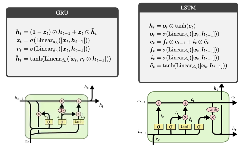
The figures might appear complicated at first. For educational purposes, let’s concentrate on the simpler one – GRU. In each round of computation, the algorithm receives:
– the input $x_t$
– the previous hidden state $h_{t-1}$
depicted by the lines incoming from the bottom and left, respectively. It outputs the new state $\mathbf h_t$, which is a linear combination of the old state $ \mathbf h_{t-1}$ and the new candidate state $\tilde{\mathbf h}_t$. The linear combination is computed in the upper line, where the old state is multiplied by $1 – \mathbf z_t$ and added to $\tilde {\mathbf h}_t$, multiplied by $\mathbf z_t$. The computation of $\mathbf z_t$ happens in the middle of the graph, where it is a processed output of the neural network with input $\mathbf x_t$ and $\mathbf h_{t-1}$, followed by a sigmoid activation function. This is called the update vector. Similarly, we compute the reset vector $\mathbf r_t$ on the left of the graph, which uses a different NN and sigmoid activation function to compute $\mathbf r_t$ from $\mathbf x_t$ and $\mathbf h_{t-1}$. The vector is then multiplied by $\mathbf h_{t-1}$, which is concatenated with $x_t$ and fed to the third NN (with a tanh activation function) to compute the candidate state $\tilde {\mathbf h}_t$ (see the outer loop at the bottom of the graph).
Clearly, the workings of GRU heavily depend on nonlinearities and recurrent connections, which makes it hard to parallelize. Despite similarities to the update equation \( \textbf{v}_k = \textbf{a}_k \odot \textbf{v}_{k-1} + \textbf{b}_k\), with \(\mathbf {v}_k = \mathbf h_k \), \(\textbf{a}_k = 1 – \textbf{z}_k\) and \(\textbf{b}_k = \textbf{z}_k \odot \tilde{\textbf{h}}_k\), both \(\textbf{z}_k\) and \(\tilde{\textbf{h}}_k\) are computed using the previous state \(\textbf{h}_{k-1}\), which makes parallel scan impossible.
Mini-GRU and Mini-LSTM
This issue is addressed in mini-GRU and mini-LSTM, where the authors have removed the recurrent connections and nonlinearities from the update and reset equations. Interestingly, this made the two architectures similar to each other, differing mainly in how they normalize the update vector.
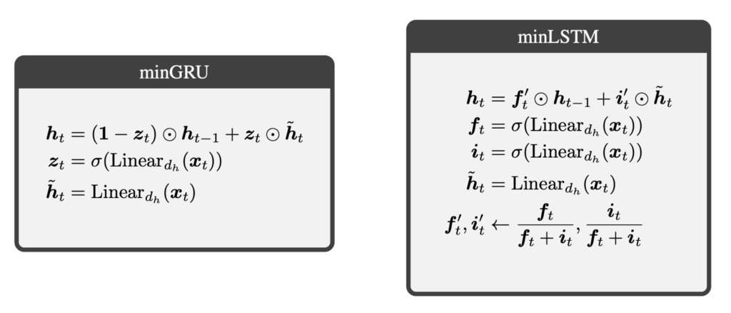
In both cases, the weights multiplying the previous state \(\mathbf h_{t-1}\) and the candidate \(\tilde{\mathbf h}_t\) add up to 1. Crucially, their computation depends only on the incoming data \(\mathbf x_t\), processed by the NN and the sigmoid activation function (mini-GRU). In mini-LSTM, there are just two NNs, computing two weights \(\mathbf f_i\) and \(\mathbf i_i\), which are normalized to sum to 1 (in the last equation). Finally, the candidate state is computed by the third NN, which again depends only on the incoming data \(\mathbf x_t\) and not on the previous state \(\mathbf h_{t-1}\).
This makes mini-GRU and mini-LSTM architectures perfectly suited for parallel scan, as the modification of the state \(\tilde {\mathbf h}_t\) can be computed in parallel from the time-series \(\mathbf x_t\) and added sequentially to the previous state \(\mathbf h_{t-1}\). We depict this mechanism for mini-GRU in the figure below:
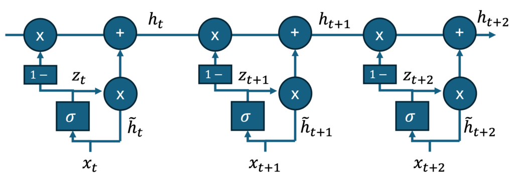
Crucially, the computation of each update block is independent, hence, for a given time series, they can be computed at the same time. Once the set of $\{\mathbf z_t, \tilde {\mathbf h}_t\}$ is computed, they are added iteratively to yield an increasingly better approximation of the state $\mathbf h_t$.
Performance
The authors report high performance of mini-GRU and mini-LSTM on a variety of sequential data processing tasks:
– Selective copy
– RL environment – MuJuCo Locomotion
– Language modeling – Shakespeare text generation
In each task, mini-GRU and mini-LSTM were compared against suitable Transformer architectures and other state-of-the-art networks, like Mamba or S4. In all cases, mini-GRU and mini-LSTM were on par with or outperformed the other architectures.
At the same time, mini-GRU and mini-LSTM are expected to consume significantly fewer resources than Transformers, which is supported by the following figure:

Context
The authors also discuss the relationship to other recent works, which is important to understand the broader context.
State-Space Models
The proposed architecture ended up being closely related to state-space models, which are used in control theory to model the dynamics of systems. A prominent example is the LTI (Linear Time-Invariant) state-space model:
\[
\mathbf x_{t+1} = \mathbf A \mathbf x_t + \mathbf B \mathbf u_t,
\]
which some of us have encountered in the context of the Kalman filter. State-space models are naturally suited to model systems governed by (possibly stochastic) differential equations, which describe most physical systems. Interestingly, data accumulation (memory) follows the same pattern.
Mamba and S4
The state-space approach has recently been used in the development of modern foundational model Mamba, which were designed to outperform Transformers in sequential data processing tasks. Although the workings of Mamba are beyond the scope of this post, it is interesting that there exists a limit where Mamba closely resembles mini-GRU and mini-LSTM:

The only difference is the lack of a linear transformation of the input data $\mathbf x_t$ in Mamba.
No Free Lunch?
As expected, mini-RNNs are not a silver bullet, though their limitations are manageable.
The main issue is memory usage, which in the investigated tasks was about 88% higher than in traditional RNNs. The additional memory is needed to store the independent blocks of \(\{\mathbf z_t, \tilde {\mathbf h}_t\}\), which are required to compute the state \(\mathbf h_t\). However, it’s worth highlighting that the memory usage is still lower than in Mamba, which consumes 56% more.
Another limitation is related to the main trick, which is casually mentioned in one of the paragraphs. For completeness, we quote the paragraph:
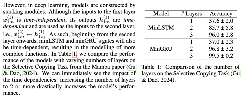
This means that more than one layer of mini-RNN is needed to represent complex temporal correlations. Although this is not a significant overhead, I would have expected this information to be emphasized more in the paper. For instance, a diagram like the one below would help clarify the concept:
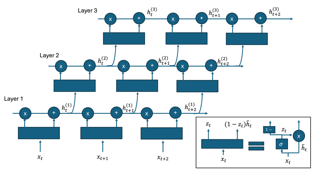
Clearly, beginning from the second layer, the gates in mini-RNNs become time-dependent.
Speculations
Comments
- Beyond the practical outcomes of the paper, it is interesting to reflect on how for decades the scientific community missed this simple solution to improve RNNs in favor of pursuing a more complicated one. Although this might seem like a trivial oversight, I believe that science often works in both directions. Sometimes we need to add more complexity to solve a particular problem in a brute-force way. Once a solution is found, the work should continue to refine it into the simplest possible form.
- It is also fascinating to think about mini-RNNs in the context of memory processes, for instance, those happening in our brains. Could it be that the brain uses a similar mechanism to store and process information? Hard to say, but the resource efficiency of mini-RNNs might suggest something along those lines. If so, the model’s ability to allow sudden changes in memory without needing to know the previous state could be significant. To make sense of this, we would expect a high-dimensional structure of \(\mathbf h_t\) that stores both short- and long-term memories on the same “tape” and a suitable form of \(\mathbf z_t\), which is typically larger for short-term and smaller for long-term memories.
Possible Applications – Edge Quantum Computers
Naturally, mini-RNNs find their application in sequential data processing tasks, where they can match the performance of Transformers with much fewer resources.
For me, the most interesting application is controlling quantum experiments, as I believe these constitute non-trivial dynamical systems. For instance, the operation of quantum computers clearly has a temporal structure, reflected in the sequential rounds of initialization, control, and measurement. Given this, leaner and more efficient mini-RNNs could potentially fit the limited resources of quantum controllers and enable more efficient operation of quantum computers. More on this soon.
